
Integrated plotting in Python#
Last major update: May, 2023
Original author: Paulo Meira
Due to the high number of images, this notebook is stored in the Git repository without outputs.
You can open and then run this notebook on Google Colab for a quick overview if you don’t want to set up a local environment: Open in Colab.
General preparation
Install Python; we recommend using miniforge from conda-forge – after installation, either create a dedicated environment or make sure the basics are installed (
conda install jupyterlab matplotlib-base ipympl scienceplots pandas)Install the DSS-Extensions (
python -m pip install dss-python[plot] opendssdirect.py)Run the following cells to download the sample DSS scripts
! git clone --depth=1 -q https://github.com/dss-extensions/electricdss-tst
fatal: destination path 'electricdss-tst' already exists and is not an empty directory.
If you are running under Google Colab, running the following cell should install the packages.
import os, subprocess
if os.getenv("COLAB_RELEASE_TAG"):
    print(subprocess.check_output('pip install dss-python[plot] opendssdirect.py[extras] ipympl scienceplots', shell=True).decode())
# Download the sample circuits and test cases
from dss.examples import download_repo_snapshot
IEEE13_PATH = download_repo_snapshot('.', repo_name='electricdss-tst', use_version=False) / 'Version8/Distrib/IEEETestCases/13Bus/IEEE13Nodeckt.dss'

assert IEEE13_PATH.exists()

print("Examples downloaded. IEEE13 file path:", str(IEEE13_PATH))
Examples downloaded. IEEE13 file path: /tmp/dss/dss_python/docs/examples/electricdss-tst/Version8/Distrib/IEEETestCases/13Bus/IEEE13Nodeckt.dss
If the download of the sample fails, and if you have Git installed, try manually running inside the same folder this notebook is located:
git clone --depth=1 -q https://github.com/dss-extensions/electricdss-tst
Otherwise, download dss-extensions/electricdss-tst and extract the electricdss-tst-master folder in the same path as this notebook. Rename it to electricdss-tst.
Introduction#
DSS-Python and OpenDSSDirect.py can use the plotting extension to enable the plot commands as seen in the official OpenDSS through our alternative implementation (currently known as DSS C-API).
The goal of this feature is to achieve similar results, but there is no intention of achieving pixel-perfect results, for various reasons.
The implementation does not reuse the concept of creation .dsv files on disk, since we avoid creating files when possible. Still, for compatibility, some features do require creating other files.
As seen in this notebook, many of the official OpenDSS examples work as-is, so you can further explore the OpenDSS documentation and examples for more.
This plotting implementation was motivated by a few points:
Provide a better (and more complete) experience for users of DSS outside of Windows, especially Linux and macOS users, but also online environments such as Google Colaboratory and JupyterHub installations.
Allow running and reusing archived OpenDSS scripts as-is. This includes some of the official OpenDSS material from EPRI, archived code repositories and datasets from users in general (e.g. results from MSc and PhD works, papers).
Allow easier customization of plots. This is a commonly requested feature.
Known issues and limitations:
The sizing of the markers may differ from the DSSView.exe; we will probably need a mapping function to address this.
Custom interactive/inspection is not implemented yet.
plot evolutionandplot energymeterare not implemented. The commanddi_plot, which is implemented, already covers some similar functionality asplot energymeter.
See also “Future development” below.
Enabling and using the plotting features#
To enable plotting, as of the May 2023, matplotlib and SciPy are required. If you don’t have them installed, you can install DSS-Python with the optional features using pip:
python -m pip install dss-python[plot]
Note that you may prefer to install the third-party packages through conda/mamba if you are using a conda environment.
Importing the plotting module (either import dss.plot or indirectly through the property Plotting) and enabling the features result in some side-effects.
Importing will register an IPython magic and some integration functions for file outputs.
Importing will set
AllowChangeDirto false.When plotting is enabled,
AllowFormsis set to true.
There are two equivalent ways to enable plotting. The first is importing the submodule and calling the enable() function:
from dss import plot
plot.enable()
The second is calling enable from a DSS instance (from DSS-Python):
from dss import dss
dss.Plotting.enable()
After enabling the features, a user can plot from the DSS-Python API, OpenDSSDirect.py API, or using the Jupyter cell magic. General matplotlib configuration applies; for example, custom figure sizes and fonts set in matplotlibrc are respected. Users can also add custom matplotlib items to complement the charts (see at the end of the Example Gallery).
As a reminder, before enabling plots, all plot ... commands from DSS scripts are ignored under DSS-Extensions.
There are a few optional arguments to the enable function that will be explored in the examples in this notebook:
? dss.Plotting.enable
Finally, if you need to disable the plotting system, there is a disable() function available.
Example using only DSS-Python#
from dss import dss
dss.Plotting.enable()
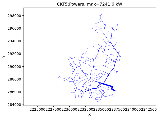
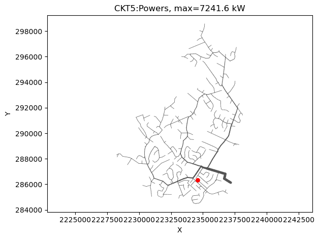
dss.Text.Command = 'redirect ./electricdss-tst/Version8/Distrib/EPRITestCircuits/ckt5/Master_ckt5.dss'
dss.ActiveCircuit.Solution.Solve()
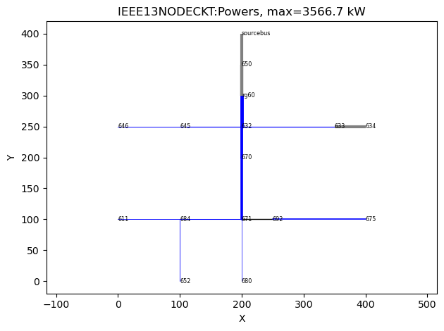
dss.Text.Command = 'plot circuit powers'
# The shorthand version would also work fine
# dss('plot circuit powers')
Example using OpenDSSDirect.py#
Remember that OpenDSSDirect.py shares the same backend as DSS-Python, so whenever you install OpenDSSDirect.py, you also install DSS-Python.
import dss.plot
import opendssdirect as odd
dss.plot.enable()
odd.Text.Command('redirect ./electricdss-tst/Version8/Distrib/EPRITestCircuits/ckt5/Master_ckt5.dss')
odd.Solution.Solve()
odd.Text.Command('plot circuit powers')
Jupyter, IPython integration and more#
Importing our plotting module on a IPython environment tries to register the %%dss cell magic. This was tested specifically for JupyterLab, but most of it works fine with Google Colaboratory.
With the cell magic, users can write DSS code directly. Unfortunately, the syntax highlighting is not yet specific to the DSS language.
%%dss

redirect somefile.dss
IDEs such as Spyder should work but the text file output is not integrated (yet?). You can use %%dss in the IPython console inside Spyder, for example, and plots will be added to the “Plots” pane.
Visual Studio Code is also a great environment for notebooks.
Since we use matplotlib, users can optionally configure the plotting backend to use SVG (vector files) instead of PNG bitmaps:
%config InlineBackend.figure_format = 'svg'
Or increase the output resolution for high DPI displays:
%config InlineBackend.figure_format = 'retina'
Sidenote: “Retina” is the marketing term used by Apple for high DPI displays. High DPI displays are in no way exclusive to Apple hardware, you can use this toggle for any 4K screen, etc.
To adjust sizes, panning and so on, one of the interactive matplotlib backends could be useful. See for example [ipympl] at https://matplotlib.org/ipympl/. Note that for local Jupyter installations, using a desktop backend usually works fine too, e.g. %matplotlib tk or %matplotlib qt works on Linux if the dependencies are installed.
Future development#
Initially, only a matplotlib backend is implemented. The matplotlib package was targeted due to its popularity, versatility and quantility of the results.
There are plans to provide alternative plotting backends someday. For example, Plotly, Bokeh and eCharts are some candidates. A Python level API will also be exposed.
We hope to implement syntax highlighting too. This will be investigated for JupyterLab 4.0. A Jupyter kernel for running pure DSS scripts could be developed to go along.
As the features mature, some of them may move to the package “AltDSS” (work-in-progress), which will provide a modern interface to our alternative DSS engine and also some niceties for the official OpenDSS engine.
Besides a few missing plots, some of the implementation ones can be polished in a future release, either by default or by toggling an option. Colormaps and colorbars are one example we should use instead of the manual colormapping in general data plots, etc.
Reading a plot from .dsv files created by the official OpenDSS could also be added. Using our full plotting backend with the official OpenDSS is not possible, but we could expose an user-friendly API to reuse our code with the official COM implementation.
Example gallery#
Let’s first enable and check the versions:
from dss import dss
dss.Plotting.enable()
print(dss.Version)
DSS C-API Library version 0.14.3 revision eb03a63a86e287bc71312d7e50c30288ae946142 based on OpenDSS SVN 3723 [FPC 3.2.2] (64-bit build) MVMULT INCREMENTAL_Y CONTEXT_API PM 20240313054323; License Status: Open
DSS-Python version: 0.15.4
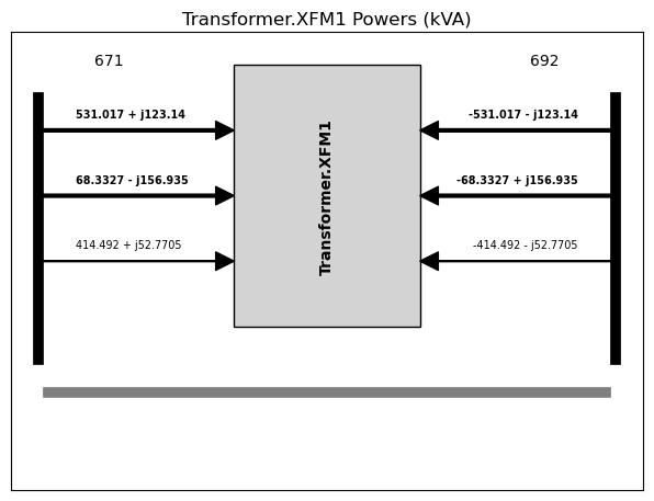
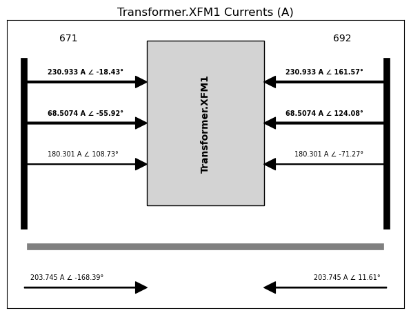
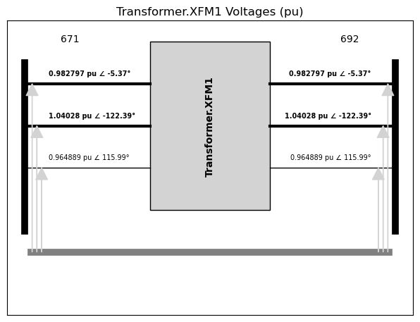
Visualize command#
# Load and solve the IEEE13 test case
dss.Text.Command = 'redirect electricdss-tst/Version8/Distrib/IEEETestCases/13Bus/IEEE13Nodeckt.dss'
dss.ActiveCircuit.Solution.Solve()
%%dss
visualize powers Transformer.xfm1
visualize currents Transformer.xfm1
visualize voltages Transformer.xfm1
Circuit plots#
Circuit plots have many variations and can be customized to add markers for the different elements and buses.
%%dss
plot circuit labels=y
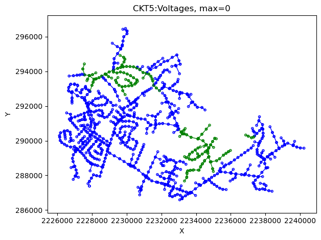
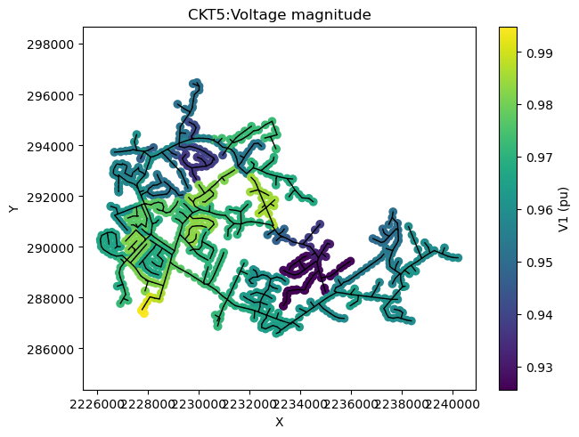
%%dss
redirect electricdss-tst/Version8/Distrib/EPRITestCircuits/ckt5/Master_ckt5.dss
set loadmult=1.5
solve
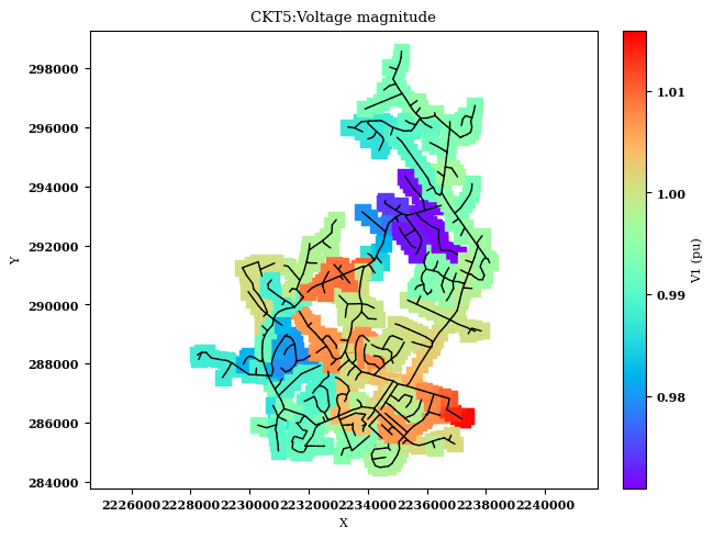
plot circuit voltage dots=n labels=n
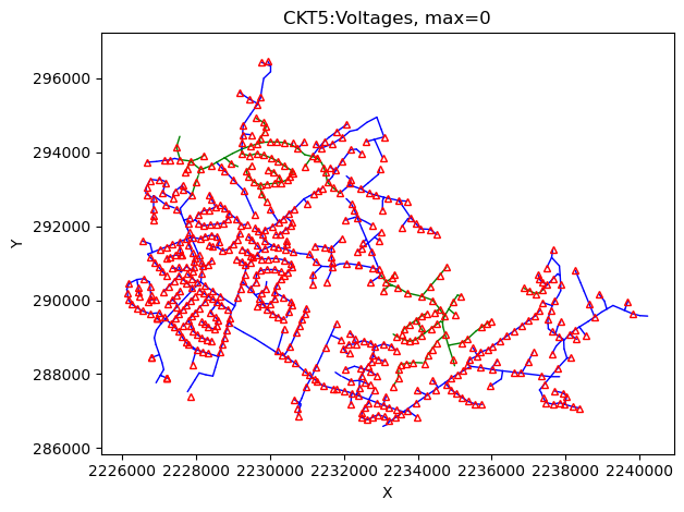
rotate -90
plot circuit voltage dots=y labels=n
set marktransformers=y
plot circuit voltage dots=n labels=n
set marktransformers=n

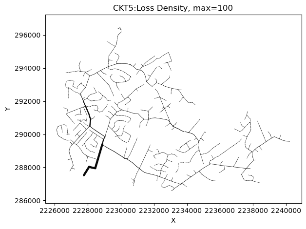
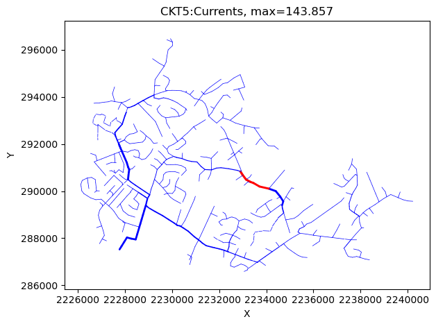
%%dss
Plot Circuit Losses 1phlinestyle=1 3phlinestyle=1 max=30
Plot Circuit Losses 1phlinestyle=2 3phlinestyle=1 max=100 c1=$0a0a0a
Plot Circuit Currents

plot scatter is one of the plot styles that would require OpenDSS Viewer:
%%dss
plot scatter
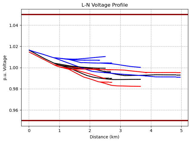
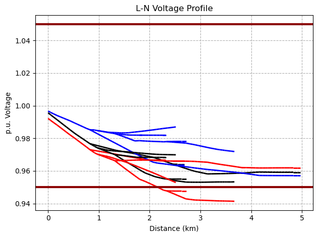
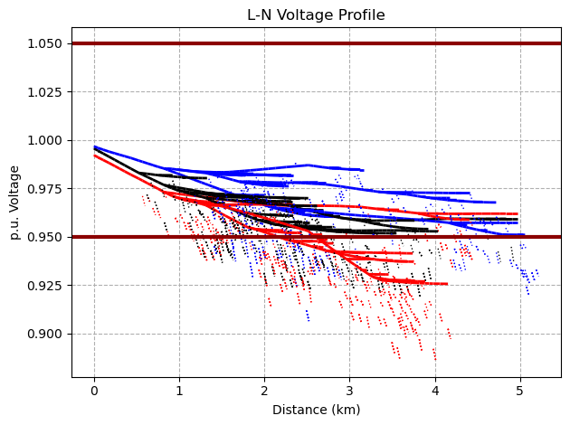
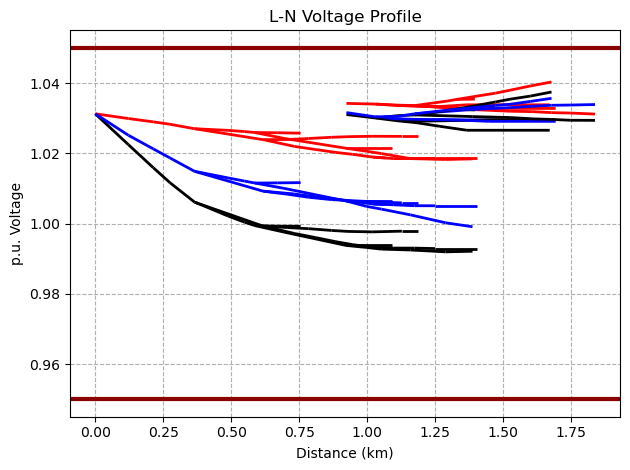
Voltage profile#
%%dss
redirect electricdss-tst/Version8/Distrib/EPRITestCircuits/ckt5/Master_ckt5.dss
solve
plot profile
set loadmult=1.5
solve
plot profile
plot profile phases=all
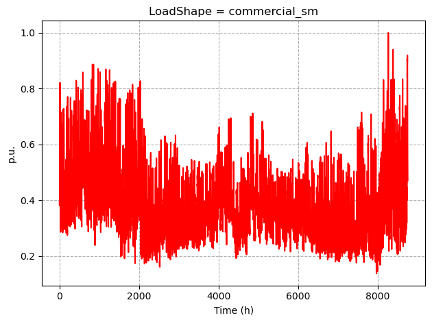
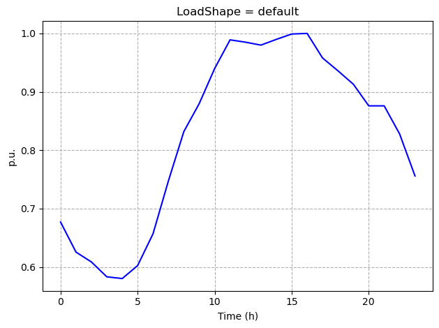
Plotting general objects#
Monitors, Loadshapes, TShapes, and PriceShapes can be plotted.
%%dss
plot loadshape object=commercial_sm c1=red
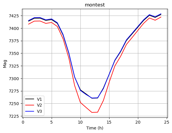
%%dss
new monitor.montest element=line.mdv201_connector
batchedit load..* daily=commercial_sm
solve mode=daily
plot monitor object=montest
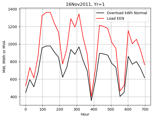
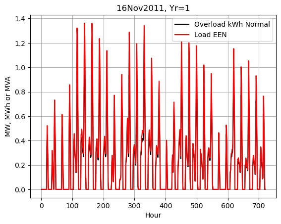
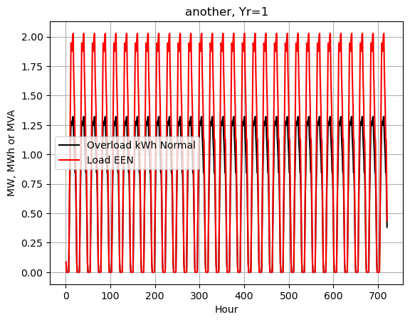
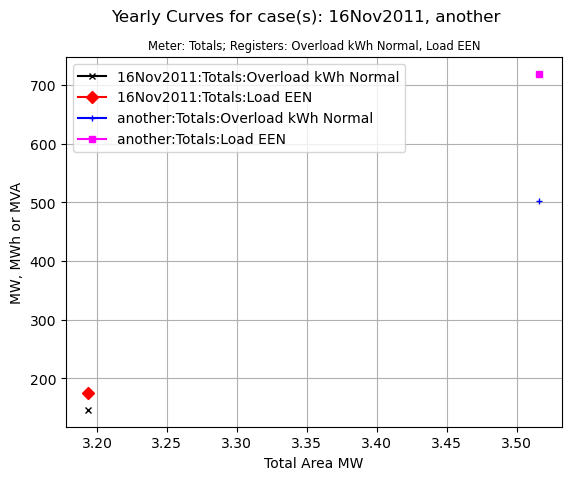
DI_plot and YearlyCurvescommands#
Note: some of these plot commands don’t seem to work with modern versions of the official OpenDSS.
# Let's disable plotting to suppress some of the output from the original script (Run_YearlySym.dss)
dss.Plotting.disable()
dss.AllowEditor = False
%%dss

// the original script already runs a scenario
redirect electricdss-tst/Version8/Distrib/IEEETestCases/123Bus/Run_YearlySim.dss

// we need a second scenario to compare later
Set CaseName=another
batchedit load..*  yearly=default
set mode=yearly number=720
Set Year=1
solve
closedi
dss.Plotting.enable()
%%dss
di_plot case=16Nov2011 registers=(9, 11) peak=y meter=DI_Totals
di_plot case=16Nov2011 registers=(9, 11) peak=n meter=DI_Totals
di_plot case=another registers=(9, 11) peak=n meter=DI_Totals
YearlyCurves cases=(16Nov2011, another) registers=(9, 11) meter=Totals
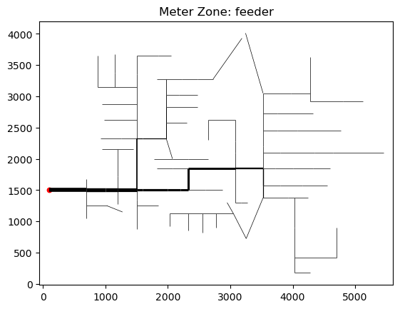
Meter Zone plot#
%%dss
Plot type=zone object=feeder quantity=power max=2000
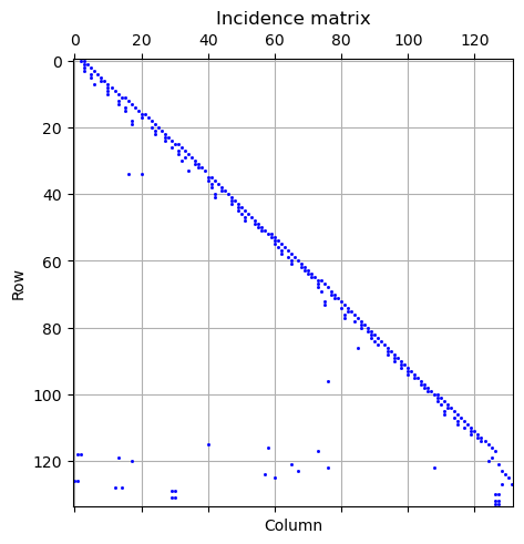
Matrix plots#
%%dss
calcincmatrix
plot matrix incidence
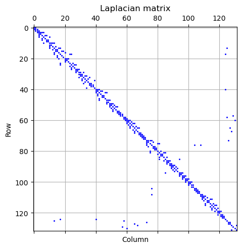
%%dss
calclaplacian
plot matrix laplacian
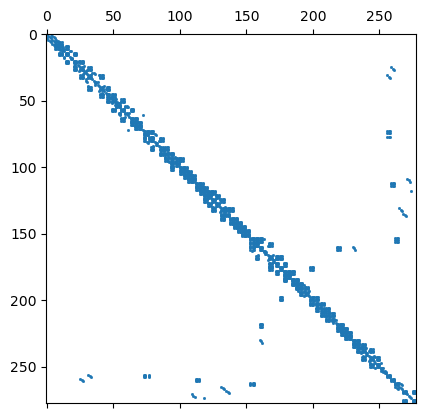
If you wish to plot the Y matrix directly, you can use the sparse version and matplotlib’s spy. For another alternative, see nschloe/betterspy
from matplotlib import pyplot as plt
from scipy.sparse import csc_matrix
Y = csc_matrix(dss.YMatrix.GetCompressedYMatrix())
plt.spy(Y, ms=1)
<matplotlib.lines.Line2D at 0x7f29d5274bf0>
3D plots#
Some plots also have 3D implementations similar to the ones available in OpenDSS Viewer (previously known as “OpenDSS Visualization Tool”).
You can enable both 2D and 3D plots where available:
dss.Plotting.enable(plot3d=True, plot2d=True)
dss.Text.Command = 'plot profile'
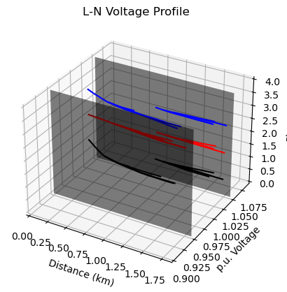
Or just the 3D plots:
dss.Plotting.enable(plot3d=True, plot2d=False)
%%dss
plot profile
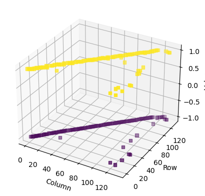
%%dss
calcincmatrix
plot matrix incidence
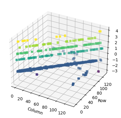
%%dss
calclaplacian
plot matrix laplacian
%%dss
plot scatter
Notebook integration: text/CSV file outputs#
Text outputs that would normally open in the editor are linked in the notebook instead. This allows the user to run a long script and then inspect the outputs more easily.
We usually recommend using the export command instead of the show command since JupyterLab includes a CSV viewer. Disabling AllowEditor silences this output message on the notebook.
dss.AllowEditor = True
%%dss
redirect electricdss-tst/Version8/Distrib/IEEETestCases/13Bus/IEEE13Nodeckt.dss
set showexport=true
export voltages
dss.AllowEditor = False
%%dss
export voltages
Following epri_dpv\DOE Tutorial.pdf#
For context, see EPRITestCircuits\epri_dpv\DOE Tutorial.pdf.
Note that some outputs changed since the original files are from 2013 and there have been changes on OpenDSS defaults and in the PVSystem model (the DSS files may have been updated too). The results presented here match the current OpenDSS release.
Used here:
circuit plots
voltage profile plots
daisy plot
general data plot
monitor plot
from dss import dss
dss.Plotting.enable()
%%dss
cd electricdss-tst/Version8/Distrib/EPRITestCircuits/epri_dpv/J1/
redirect "Master_noPV.dss"
solve
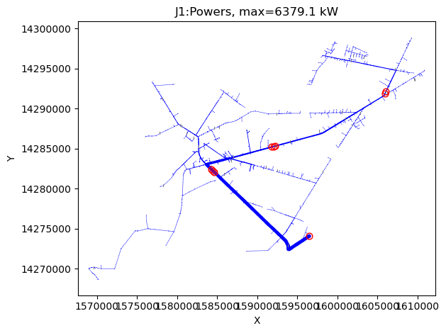
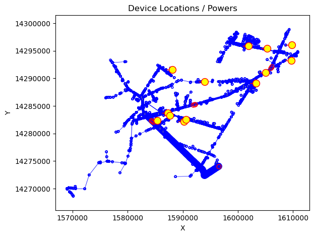
Plot Circuit Power flow
%%dss
set markercode=24
set markregulators=yes
plot circuit power 1ph=3
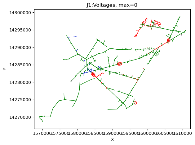
Plot voltages
%%dss
set emergvminpu=1.0
set normvminpu=1.035
plot circuit voltage
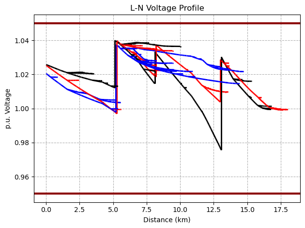
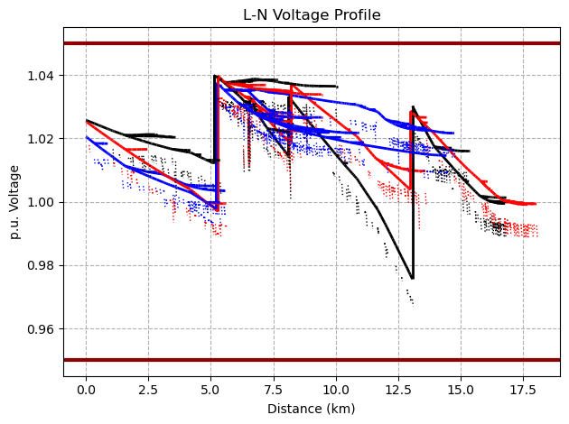
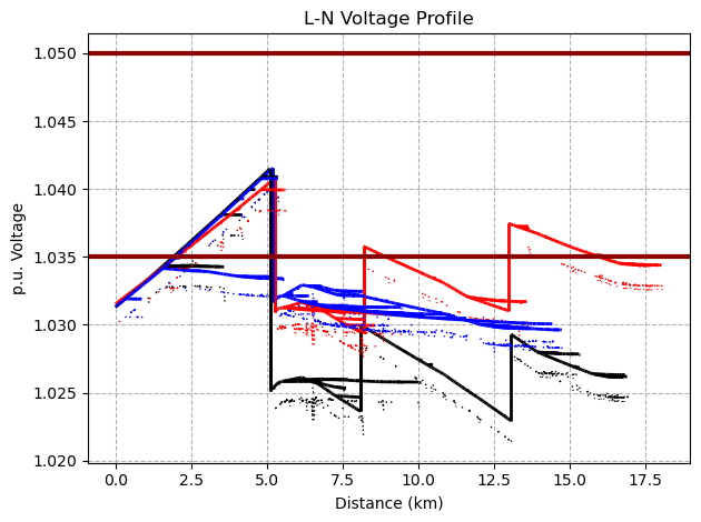
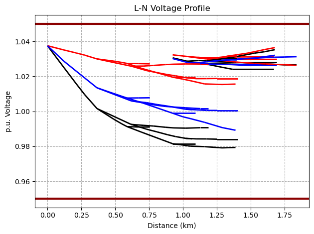
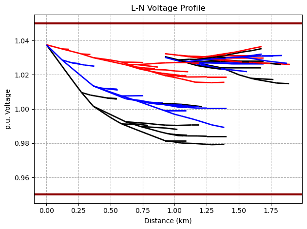
Plot profile
%%dss
set normvminpu=0.95
plot profile phases = primary
plot profile phases = all
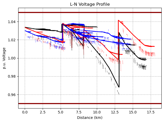
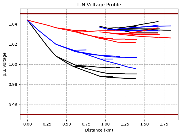
Minimum load case (approximate)
%%dss
set emergvminpu=1.0
set normvminpu=1.035
set loadmult=.1
solve
plot profile phases = all
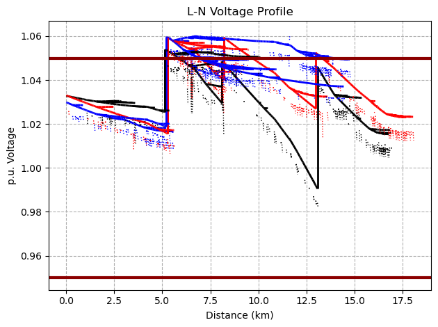
Add PV to Circuit Model
%%dss
clear
redirect Master_noPV.dss
solve

Redirect ExistingPV.dss
Set DaisySize=2.5
set markregulators=yes
plot daisy power max=2000 dots=y buslist=(file=PVbuses.txt)

solve
plot profile phases=all
Compare saved voltages to current case solved
%%dss
redirect "Master_noPV.dss"
solve
save voltages
Redirect ExistingPV.dss
! Disable all controls
set controlmode=off
solve
plot profile phases=all
vdiff ! creates voltage difference file
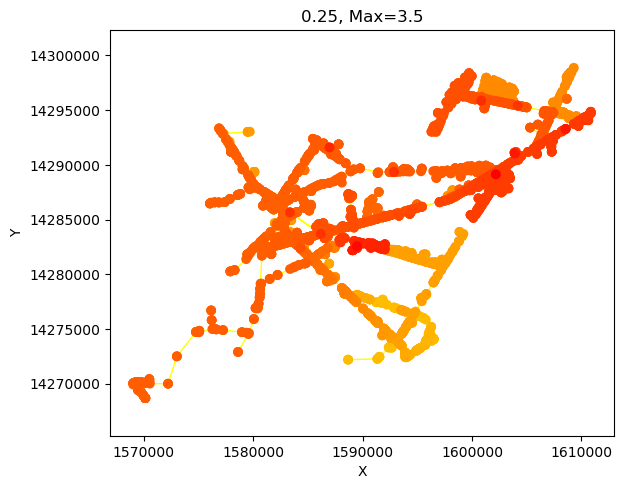
set markercode=24 nodewidth=2.5
! Plot difference in voltage between no-PV and with-PV cases
plot general quantity=1 max=3.5 min=0.0 C1=$0000FFFF C2=$000000FF dots=y labels=n object=electricdss-tst/Version8/Distrib/EPRITestCircuits/epri_dpv/J1/J1_VDIFF.txt
Run time series analysis
%%dss
compile Master_noPV.dss
Redirect ExistingPV.dss
solve
new loadshape.mypv npts=1800 sinterval=1 csvfile=StrwPlns1sec30min.csv
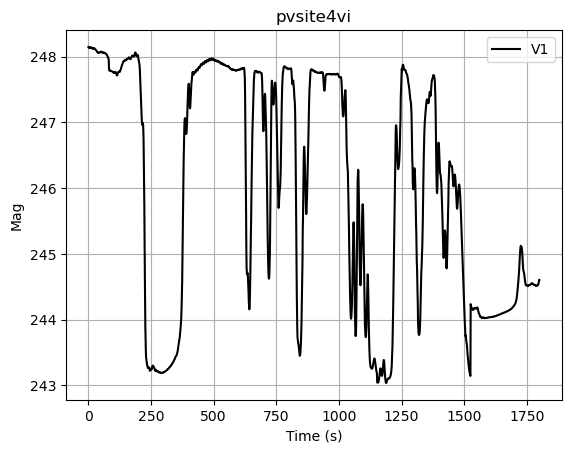
new monitor.PVSite4VI element=PVSystem.3P_ExistingSite4 terminal=1 mode=0
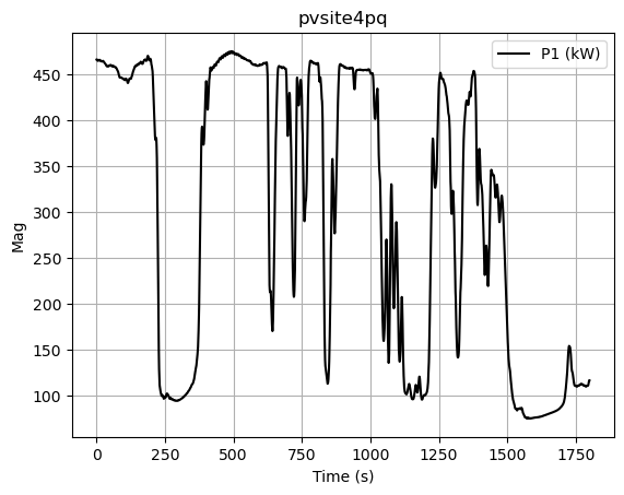
new monitor.PVSite4PQ element=Line.Site4_PV terminal=2 mode=65 ppolar=no
! Assign same PV curve to all PV systems (single curve used for demo only)
batchedit pvsystem..* daily=mypv
solve mode=daily stepsize=1s number=1800
batchedit pvsystem..* pf=-0.98
! Plotting
plot monitor object=pvsite4vi channels=(1 )
plot monitor object=pvsite4pq channels=(1 )
Restore the current dir in the DSS engine
%%dss
cd ../../../../../..
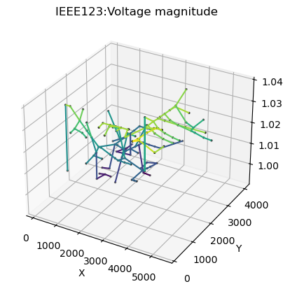
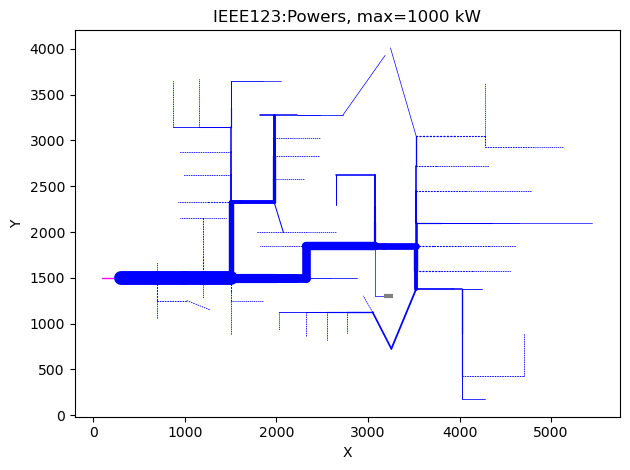
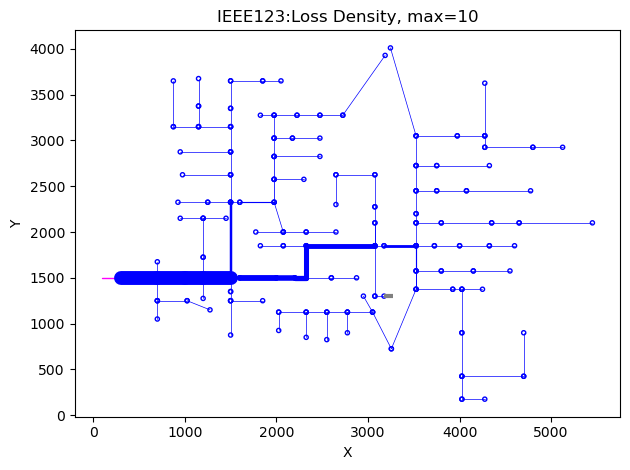
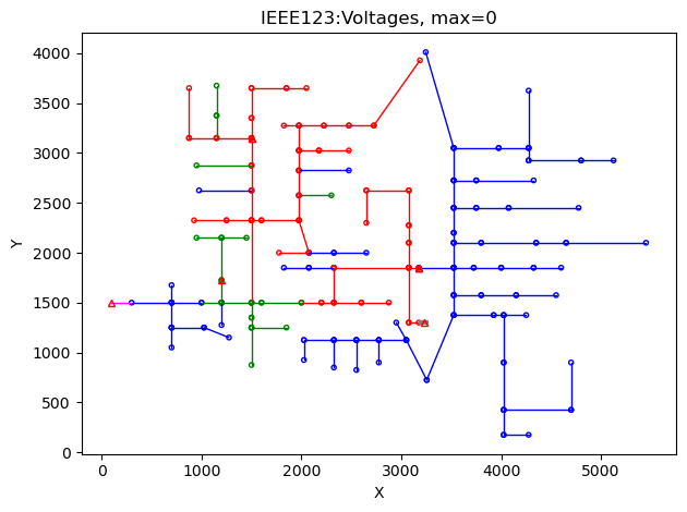
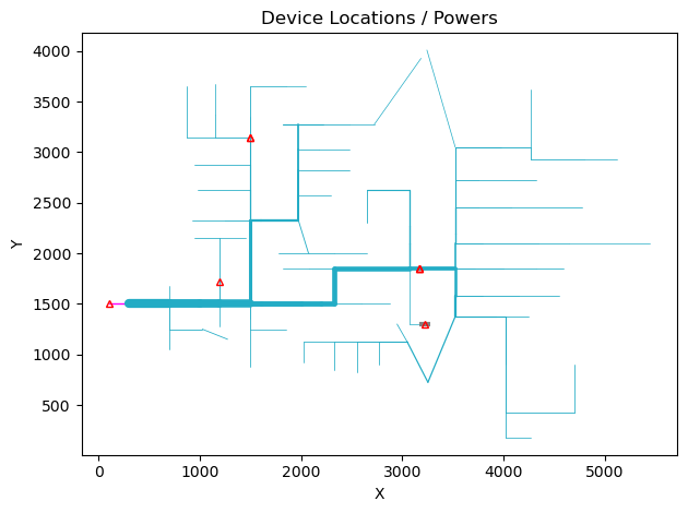
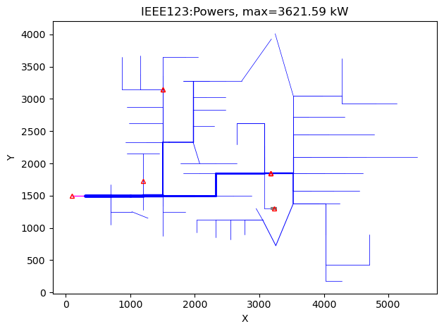
Running the IEEE123 sample script#
This is one of the OpenDSS sample scripts. We invite users to run the same files on the official OpenDSS to compare and validate the output here. For file outputs, note that if the circuit or casename are not changed, the previous files are overwritten (just like in the official OpenDSS). We could modify the script to address that, but let’s focus on the plots for now. A future release may handle reports better.
If you wish to inspect the scripts, uncomment the contents of the following cell:
# from pathlib import Path
# print(Path('./electricdss-tst/Version8/Distrib/IEEETestCases/123Bus/Run_IEEE123Bus.DSS').read_text())
# print(Path('./electricdss-tst/Version8/Distrib/IEEETestCases/123Bus/CircuitPlottingScripts.dss').read_text())
%%dss
redirect ./electricdss-tst/Version8/Distrib/IEEETestCases/123Bus/Run_IEEE123Bus.DSS
redirect ./electricdss-tst/Version8/Distrib/IEEETestCases/123Bus/CircuitPlottingScripts.dss
Saving the outputs#
Currently we don’t provide a way to autosave the outputs, especially since a notebook already comprises the basics of that functionality.
If you think autosaving to separate files would be good for users in general, please voice your opinion by opening an issue at dss-extensions/dss_python
On a notebook, to manually save, you can disable the auto-show option. This will keep the figures open so you can interact with them before discarding the results. You will note that the figures are still automatically shown, but the output order may change (that’s why we don’t use show=False as a default).
from matplotlib import pyplot as plt

dss.Plotting.enable(show=False)
dss.Text.Command = 'plot circuit'
plt.savefig('circuit.svg')
dss.Plotting.enable(show=True)
Customizing the figures#
The output can be customized in many ways:
Exporting to third-party software (e.g. use Inkscape to complement SVG files)
Through the DSS commands: enabling and choosing markers, colors, etc.
Through matplotlib’s general options: see https://matplotlib.org/stable/tutorials/introductory/customizing.html – you can set default fonts, sizes, and various other aspects of the figures.
Through matplotlib’s API: adding custom elements to the intermediate output
Applying matplotlib styles#
Here’s a short example of using different matplotlib styles. See also https://matplotlib.org/stable/gallery/style_sheets/style_sheets_reference.html
from matplotlib import pyplot as plt
from dss import dss
dss.Plotting.enable(show=False)
dss.Text.Command = 'redirect electricdss-tst/Version8/Distrib/EPRITestCircuits/ckt5/Run_ckt5.dss'
dss.ActiveCircuit.Solution.Solve()
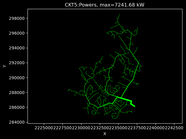
with plt.style.context('dark_background'):
dss.Text.Command = 'plot circuit c1=lime'
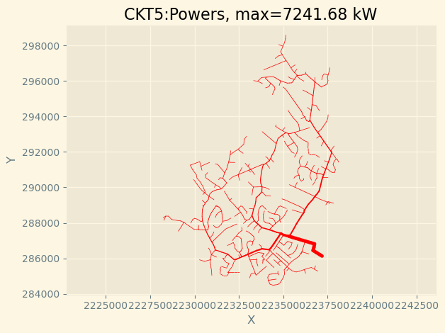
with plt.style.context('Solarize_Light2'):
dss.Text.Command = 'plot circuit c1=red'
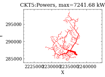
For more styles, install SciencePlots (available through conda or pip): garrettj403/SciencePlots
try:
    import scienceplots
    with plt.style.context(['science', 'no-latex']): # if you have LaTeX installed, remove 'no-latex'
        dss.Text.Command = 'plot circuit c1=red'
except:
    # let's ignore if the user didn´t install SciencePlots
    pass
Adjusting specific elements#
If using a style is not desired, users can adjust specific elements. rc_context is a way to control the elements temporarily, while rcParams allow changing the params for the current session.
from matplotlib import rc_context

with rc_context({
    'font.size': 8,
    'font.family': 'Serif',
    'font.weight': 'bold',
    'scatter.marker': 's',
    'lines.markersize': 10,
    'image.cmap': 'rainbow',
}):
    dss('plot scatter')
Customizing using matplotlib’s API#
As in the previous example for saving the figure, we will disable auto-show so we can interact with the figures, and then add some extra elements.
from matplotlib import pyplot as plt
from dss import dss

dss.Plotting.enable(show=False)

# We'll use the EPRI ckt5 test circuit here
dss.Text.Command = 'redirect electricdss-tst/Version8/Distrib/EPRITestCircuits/ckt5/Run_ckt5.dss'

# Select a bus
name = '820'
bus = dss.ActiveCircuit.Buses[name]
x, y = bus.x, bus.y
print('Selected bus:', name)
Selected bus: 820
As a reminder, if you just need to add a marker quickly, you could just use a simple bus marker:
dss.Text.Command = 'ClearBusMarkers' # remove the previous marker
dss.Text.Command = f'AddBusMarker Bus={name} code=24 color=red size=5'
dss.Text.Command = 'plot circuit c1=$555555'
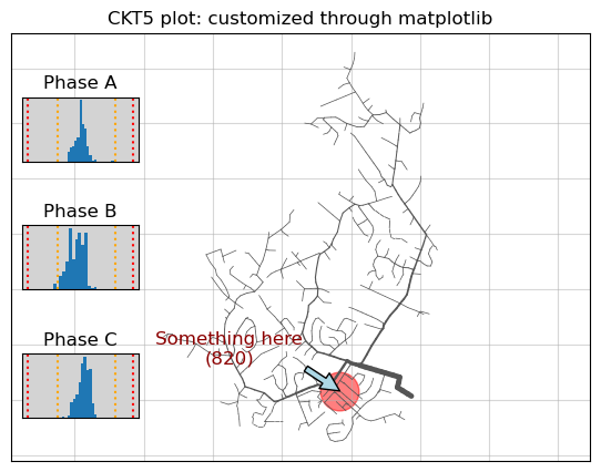
Alternatively, let’s customize the output to add a marker and some tiny histograms.
dss.Text.Command = 'ClearBusMarkers' # remove the previous marker
dss.Text.Command = 'plot circuit c1=$555555'

# Point to the select bus
plt.annotate(f"Something here\n({name})", (x,  y), xytext=(x - 4000, y + 1000), arrowprops=dict(fc='lightblue'), fontsize='larger', ha='center', color='darkred')
plt.plot(x, y, 'o', color='red', ms=25, zorder=-10, alpha=0.5)

# Show grid, hide the axis (spines and labels)
plt.grid(alpha=0.5)
plt.tick_params(labelleft=False, left=False, bottom=False, labelbottom=False)

# Change the title and remove labels
plt.title('CKT5 plot: customized through matplotlib')
plt.xlabel('')
plt.ylabel('')

# Add a few voltage histograms, one per phase
for ph in (1, 2, 3):
    ax = plt.gca().inset_axes([0.02, 0.7 - 0.3 * (ph - 1), 0.2, 0.15])
    ax.set_facecolor('lightgray')
    ax.hist(dss.ActiveCircuit.AllNodeVmagPUByPhase(ph), bins=20)
    ax.tick_params(labelleft=False, left=False, bottom=False, labelbottom=False)
    ax.axvline(dss.ActiveCircuit.Settings.NormVmaxpu, color='orange', ls=':')
    ax.axvline(dss.ActiveCircuit.Settings.NormVminpu, color='orange', ls=':')
    ax.axvline(dss.ActiveCircuit.Settings.EmergVminpu, color='r', ls=':')
    ax.axvline(dss.ActiveCircuit.Settings.EmergVmaxpu, color='r', ls=':')
    ph_name = 'ABC'[ph - 1]
    ax.set_title(f'Phase {ph_name}')
# Toggle auto-showing back
dss.Plotting.enable(show=True)